A seamless approach
The approach adopted here is to document the state of the atmosphere and the ocean through a continuum of scales ranging from seasonal to monthly and ending at the scale of the storm system. The interest is to place the meteorological situation of the day or week in a large-scale context that may or may not provide predictability.
Seasonal scale:
More specifically, it is a question of starting the analysis with observations on the largest scales in terms of global and seasonal means and then analysing their seasonal forecast.
Sub-seasonal scale:
The analysis for the sub-seasonal forecast allows to identify the trends within a season and eventually to confirm or amend the results of the seasonal forecast. The objective here is to anticipate the onset of the rainy season (delayed, early arrival), the wetter or drier phases during the full monsoon and the end of the season (delayed, early end).
Synoptic scale:
Synoptic forecasting makes it possible to go to a finer, deterministic scale, a few days ahead. The challenge is to anticipate the occurrence of precipitating systems in the context provided by the sub-seasonal and seasonal analyses. The focus is on extreme rainfall events.
This methodology is adopted for weekly briefings with a time devoted to each scale. The complementary websites are as follows: LIST TO BE COMPLETED
Intra-seasonal anomalies and raw fields
The intra-seasonal anomaly work is at the core of MISVA. It corresponds to the implicit mental work performed by an experienced forecaster when analysing a wind or temperature map. As the fields are very smooth and slowly evolving, the forecaster builds his own climatology and removes it from what he sees on the screen.
The MISVA products make this approach objective by calculating the intraseasonal anomaly of the most important parameters (Precipitable Water, Velocity Potential, Wind, Temperature) as follows
Computation of a smoothed annual cycle: A daily climatological annual cycle is computed over the period [1990-2020]. This corresponds to a daily average smoothed to retain only the variability of the annual cycle, i.e. retaining only periods longer than 120 days. To do this, a Fourier filtering is performed on the daily annual cycle, retaining only the first 3 harmonics (c.f. Wheeler and Kiladis 1999).
Computation of the intra-seasonal anomaly: This is the anomaly associated with scales smaller than the smoothed annual cycle. It is calculated by subtracting the smoothed climatological mean described above from the day’s parameters. The intra-seasonal anomaly makes it possible to follow the propagation of waves or variability modes that will modulate the environment and the occurrence of convective systems.
Example on a rainfall time series:
On the figure opposite, we take the example of the average rainfall in the Central Sahel. The smoothed annual cycle corresponds to the short green curve. It shows a slow evolution during the season.
In the example opposite, days where the daily rainfall (grey) is above the smoothed annual cycle (green) have a positive rainfall anomaly and conversely, days where the grey bars are below the green curve have a negative anomaly. The orange curve represents the annual cycle of the current year.

“Object” approach to gain predictability
We then try to follow the evolution of important meteorological objects (African Easterly wave, thermal depression) for the occurrence of convective systems by considering the most appropriate parameters from which a set of specific products has been developed. One of the difficulties in forecasting convective systems in West Africa is the poor performance of numerical forecast models in predicting daily rainfall. This difficulty is overcome by using both :
- a meteorological “object” approach, which makes it possible to follow in time and space an easterly wave or a wet anomaly for example. The most important objects are detailed here.
- parameters with more predictability than the predicted rainfall, such as precipitable water or velocity potential, on the basis of which the specific products have been constructed.
A documentation of the most effective parameters and products that a forecaster should master is available here.
The most effective products on the MISVA site are built in this spirit. They are based on parameters that bring more predictability than the forecasted rainfall and the superposition of several information on a given weather object. They are detailed in this page and constitute a solid basis on which a forecaster can rely on.
Temporal filtering
The intra-seasonal anomalies obtained are the result of a superposition of different temporal scales ranging from the diurnal cycle, to the modulation of the African Easterly waves to the Madden-Julian Oscillation. A simple way to separate these scales is to perform a temporal (frequency) filtering allowing to pass the high frequencies (1/T> 1/ 10 days), the low frequencies (< 1/30 days) or to isolate the intermediate frequencies between 10 and 30 days.
Spatial and Temporal filtering
A more powerful approach is to filter the intra-seasonal anomalies both in time and space to isolate the contribution of equatorial waves. The methodology of Wheeler and Kiladis (1999) and Wheeler and Hendon (2004) is used and detailed below.
A time series of 360 days of observations followed by 10 days of forecasts (in the case of the deterministic model) is constructed at each point of latitude and longitude and then completed by 180 days containing the climatology. The intraseasonal anomaly is constructed by subtracting an annual daily climatological cycle in which only the first 3 harmonics are retained (T> 120 days).
A Fourier transform is performed in time and space on the intra-space anomaly to project the parameter into wave number-frequency space. In the process of filtering a given wave, the values of the parameter are set to zero for all wavenumbers and frequencies except in the value ranges where that wave is defined.
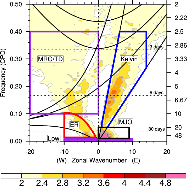
The filter domains are presented below for each wave with the spectrum of the OLR spectral density (i.e. the variance of the OLR obtained for each wavenumber). The periods (T) and wave numbers (k) considered for each wave are also shown.
- Purple : low frequency:
- T > 120 days, – 10 < k < 10
- Black : Maden-Julian Oscillation (MJO) :
- 30 days < T < 96 days, 0 < k < 9
- Red : Equatorial Rossby wave (ER)
- : 9,7 days < T < 72 days , -10 < k < -1
- Blue : Kelvin wave (K) :
- 2,5 days < T < 17 days, 1< k < -14
- Green : TD/MRG :
- 2.5 days < 7 < 10 days , -20 < k < -6