Description
This product is available at Prévision Synoptique Hovmollers – Misva (aeris-data.fr) with the following selection : Domain = Global ; Parameter = PW-VelPot-Stream-Fct and for different choices of latitude bands for the deterministic forecast and at Hovmollers_Monthly – Misva (aeris-data.fr) for the ensemble subsaisonnal forecast with a wide choice of variables (Parameter= Vel-Pot-200, PW, Uwind-850…). It shows the evolution in time (y-axis) and longitude (x-axis) of the intraseasonal anomaly of a parameter in a range of colours superimposed on the convection-favourable contributions of each equatorial wave (solid contour). The fields plotted are averages over a latitude band ([5°N-15°N] for example) based on daily data. It is advisable to start with the sub-seasonal forecast hovmöller (for precipitable water and zonal wind at 850 hPa) to get a “long-term” view, then analyse the hovmöllers on the deterministic forecast for a D-D+10 view. This gives the general trend for the current week. The example below shows the product combining these hovmöllers for the velocity potential at 200 hPa (left), the streamfunction at 200 hPa (centre) and precipitable water (right). The analysis of deterministic hovmöllers, which provides the essential elements, is detailed here. The analysis of each of these parameters is described in more detail below. Time flows from top to bottom, with the boundary between observation and forecast represented by the dotted horizontal line.

This figure is to be combined with wave superposition maps for the velocity potential at 200 hPa (detailed under Contributions of Equatorial Waves to anomalies – Misva (aeris-data.fr).
Suggested methodology
The contributions of each wave are identified by filtering the observation and model data in space (wave number) and time (frequency) using the method of Wheeler and Kiladis (1999) and Wheeler and Handon (2004).
A time series of 360 days of observations followed by 10 days of forecasts (in the case of the deterministic model) is constructed for each point of latitude and longitude and then completed by 180 days containing the climatology. The intraseasonal anomaly is constructed by subtracting an annual daily climatological cycle in which only the first 3 harmonics are retained (T> 120 days).
A Fourier transform is performed in time and space on the intraseasonal anomaly to project the parameter into wavenumber-frequency space. During the filtering process for a given wave, the parameter values are set to zero for all wavenumbers and frequencies except in the value intervals where this wave is defined.
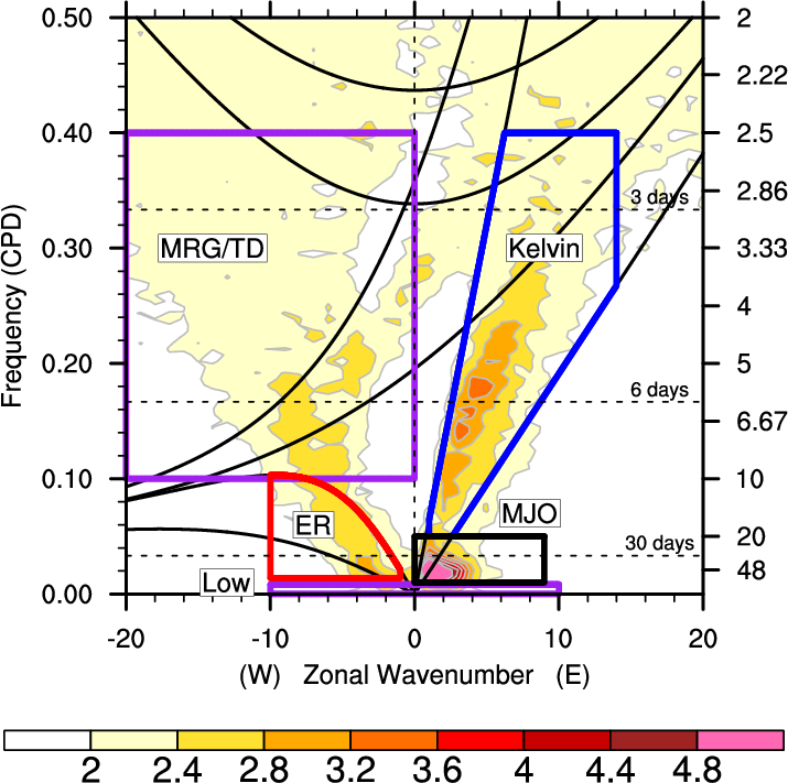
The filtering domains are shown below for each wave with the spectrum of the OLR spectral density (i.e. the variance of the OLR obtained for each frequency-wavenumber). The periods (T) and wavenumbers (k) considered for each wave are also indicated.
- Purple : low frequency
- T > 120 days, – 10 < k < 10
- Black : Maden-Julian Oscillation (MJO)
- 30 days < T < 96 days, 0 < k < 9
- Red : Onde de Rossby équatoriale (ER)
- : 9,7 days < T < 72 days , -10 < k < -1
- Bleu : Onde de Kelvin (K)
- 2,5 days < T < 17 days, 1< k < 14
- Green : Tropical Depression and Mixed Rossby Wave – TD/MRG
- 2.5 days < T < 10 days , -20 < k < -6
Use of the Velocity Potential at 200 hPa
Velocity Potential Hovmöller
The example opposite shows a hovmöller velocity potential at 200 hPa. The blue/green colours indicate an altitude divergence that is more marked than normal, favourable or indicative of deep convection. Brown areas indicate subsidence anomalies, unfavourable for convection.
This figure can be analysed as follows:
If we look first at the low frequency (purple outline), we can see a dipole of enhanced divergence at 90°E and subsidence at 60°W. The location and intensity of the low frequency can strongly modulate wave activity. In this case, it will be over the Indian Ocean and the tropical Atlantic, but little over West Africa.
We then analyse the displacement of the MJO, which is generally quite clear on this parameter. We detected the propagation of a negative, subsident phase (black dashed line), which began on 8/09 at 120°W and propagated eastwards to the analysis line (horizontal line on 28/10). An active convection phase (solid black line) is also visible at 120°W, which is initially fairly stationary (the contour remains at the same longitude) and then propagates towards 15°W on 27/10.
We can also see the propagation of an upper level divergence anomaly completely to the left of the graph, on 3/10 at 180°W and propagating eastwards (downwards and to the right) to reach 15°W around 27/10. It is associated with a blue contour, i.e. a Kelvin wave, which is known to be well marked in divergence/convergence and to favour large convective systems.

Finally, we also note that this anomaly crosses a wave moving westwards, shown in red: this is an equatorial Rossby wave. We are following the evolution of the structures in the forecasts, with the Kelvin wave which is continuing to be very marked. From a forecaster’s point of view, we can expect a strengthening of the convection during the whole path of the Kelvin wave with a peak of activity at least at the crossing of the equatorial Rossby wave.
Streamfunction Hovmöller
The hovmöller of the streamfunction opposite is complementary but more difficult to interpret because it depends on the latitude band, which must be selected with the help of the equatorial wave decomposition maps available under Wave_filtered_Maps – Misva (aeris-data.fr). This variable is well-suited to detecting Kelvin and Rossby waves, confirming the previous analysis based on the velocity potential. In this case, we can clearly see the intersection of these two waves near the Atlantic coast.

Use of the Precipitable Water
A good complement to the study of the velocity potential at 200 hPa – a dynamic factor favouring convection – is to use precipitable water, another important ingredient in favouring convection. The hovmöller opposite continues with the previous example. As you can see, the structures are not the same as for the velocity potential and the streamfunction, because each wave has a different signature in terms of divergence, eddy, circulation or humidity. For the precipitable water parameter, it is mainly the equatorial Rossby waves that can be detected, as well as the effect of the low frequency. The red outline shows the propagation of an equatorial Rossby wave, earlier than with the Velocity Potential hovmöller. It starts at 90°E on 23/09 and reaches West Africa on 20-28/10. Detecting and tracking this type of signal brings predictability to the situation and adds to the strong altitude divergence mentioned on the Velocity Potential hovmöllerl, a high humidity compared to the climatology.

Additional products
The equatorial wave hovmöllers derived from the sub-seasonal forecasts are interpolated on the same basis. They represent the intraseasonal anomaly of the forecast ensemble mean (51 members). In particular, they provide a long-range view (6 weeks) to which the MJO and equatorial Rossby waves can make a major contribution. In the case presented above, the hovmöllers of precipitable water made it possible to anticipate the arrival of the equatorial Rossby wave a few weeks in advance.